Manual
Rack
Plugin Development
- Tutorial
- API Guide
- Panels
- Manifest
- Presets
- Voltage Standards
- Digital Signal Processing
- Migrating v1 Plugins to v2
- Licensing
Rack Development
Appendix
Digital Signal Processing
Digital signal processing (DSP) is the field of mathematics and programming regarding the discretization of continuous signals in time and space. One of its many applications is to generate and process audio from virtual/digital modular synthesizers.
There are many online resources and books for learning DSP.
- Digital signal processing Wikipedia: An overview of the entire field.
- Julius O. Smith III Online Books (Index): Thousands of topics on audio DSP and relevant mathematics, neatly organized into easy-to-digest but sufficiently deep pages and examples.
- Seeing Circles, Sines, and Signals: A visual and interactive introduction to DSP.
- The Scientist and Engineer’s Guide to Digital Signal Processing by Steven W. Smith: Free online book covering general DSP topics.
- The Art of VA Filter Design (PDF) by Vadim Zavalishin: Huge collection of deep topics in digital/analog filter design and analog filter modeling.
- DSPRelated.com: Articles, news, and blogs about basic and modern DSP topics.
- Digital Signal Processing MIT OpenCourseWare: Video lectures and notes covering the basics of DSP.
- KVR Audio Forum - DSP and Plug-in Development: Music DSP and software development discussions.
- Signal Processing Stack Exchange: Questions and answers by thousands of DSP professionals and amateurs.
The following topics are targeted toward modular synthesizer signal processing, in which designing small but precise synthesizer components is the main objective.
This document is currently a work-in-progress. Report feedback and suggestions to VCV Support. Image credits are from Wikipedia.
Signals
A signal is a function
Analog hardware produces and processes signals, while digital algorithms handle sequences of samples (often called digital signals.)
Fourier analysis
In DSP you often encounter periodic signals that repeat at a frequency
As it turns out, not only periodic signals but all signals have a unique decomposition into shifted cosines.
However, instead of integer harmonics, you must consider all frequencies
For a digital periodic signal with period
The fast Fourier transform (FFT) is a method that surprisingly computes the DFT of a block of
Sampling
The Nyquist–Shannon sampling theorem states that a signal with no frequency components higher than half the sample rate
In practice, analog-to-digital converters (ADCs) apply an approximation of a brick-wall lowpass filter to remove frequencies higher than
Digital-to-analog converters (DACs) convert a digital value to an amplitude and hold it for a fraction of the sample time. A reconstruction filter is applied, producing a signal close to the original bandlimited signal. High-quality ADCs may include digital upsampling before reconstruction. Dithering may be done but is mostly unnecessary for bit depths higher than 16.
Of course, noise may also be introduced in each of these steps. Fortunately, modern DACs and ADCs as cheap as $2-5 per chip can digitize and reconstruct a signal with a variation beyond human recognizability, with signal-to-noise (SNR) ratios and total harmonic distortion (THD) lower than -90dBr.
Aliasing
The Nyquist–Shannon sampling theorem requires the original signal to be bandlimited at
Consider the high-frequency sine wave in red. If the signal is sampled every integer, its unique reconstruction is the signal in blue, which has completely different harmonic content as the original signal. If correctly bandlimited, the original signal would be zero (silence), and thus the reconstruction would be zero.

A square wave has harmonic amplitudes

The curve produced by a bandlimited discontinuity is known as the Gibbs phenomenon.
A DSP algorithm attempting to model a jump found in sawtooth or square waves must include this effect, such as by inserting a minBLEP or polyBLEP signal for each discontinuity.
Otherwise, higher harmonics, like the high-frequency sine wave above, will pollute the spectrum below
Even signals containing no discontinuities, such as a triangle wave with harmonic amplitudes
The most general approach is to generate samples at a high sample rate, apply a FIR or polyphase filter, and downsample by an integer factor (known as decimation).
For more specific applications, more advances techniques exist for certain cases. Anti-aliasing is required for many processes, including waveform generation, waveshaping, distortion, saturation, and typically all nonlinear processes. It is sometimes not required for reverb, linear filters, audio-rate FM of sine signals (which is why primitive digital chips in the 80’s were able to sound reasonably good), adding signals, and most other linear processes.
Linear filters
A linear filter is a operation that applies gain depending on a signal’s frequency content, defined by
A log-log plot of

To be able to exploit various mathematical tools, the transfer function is often written as a rational function in terms of
To digitally implement a transfer function, define
A first order approximation of this is
This is known as the Bilinear transform.
In digital form, the rational transfer function is written as
The zeros of the filter are the nonzero values of
We should now have all the tools we need to digitally implement any linear analog filter response
IIR filters
An infinite impulse response (IIR) filter is a digital filter that implements all possible rational transfer functions.
By multiplying the denominator of the rational
For
FIR filters
A finite impulse response (FIR) filter is a specific case of an IIR filter with
Long FIR filters (
While the naive FIR formula above requires
Impulse responses
Sometimes we need to simulate non-rational transfer functions.
Consider a general transfer function
The signal
Repeating this process in the digital realm gives us the discrete convolution.
Brick-wall filter
An example of a non-rational transfer function is the ideal lowpass filter that fully attenuates all frequencies higher than
The inverse Fourier transform of
Windows
Like the brick-wall filter above, many impulse responses
TODO
Minimum phase systems
TODO
MinBLEP
TODO
PolyBLEP
TODO
Circuit modeling
Although not directly included the field of DSP, analog circuit modeling is necessary for emulating the sound and behavior of analog signal processors with digital algorithms. Instead of evaluating a theoretical model of a signal processing concept, circuit modeling algorithms simulate the voltage state of physical electronics (which itself might have been built to approximate a signal processing concept.) Each component of a circuit can be modeled with as little or as much detail as desired, of course with trade-offs in complexity and computational time.
Before attempting to model an circuit, it is a good idea to write down the schematic and understand how it works in the analog domain. This allows you to easily omit large sections of the circuit that offer nothing in sound character but add unnecessary effort in the modeling process.
Nodal analysis
TODO
Numerical methods for ODEs
A system of ODEs (ordinary differential equations) is a vector equation of the form
The study of numerical methods deals with the computational solution for this general system. Although this is a huge field, it is usually not required to learn beyond the basics for audio synthesis due to tight CPU constraints and leniency for the solution’s accuracy.
The simplest computational method is forward Euler.
If the state
Optimization
After implementing an idea in code, you may find that its runtime is too high, reducing the number of possible simultaneous instances or increasing CPU usage and laptop fan speeds. There are several ways you can improve your code’s performance, which are listed below in order of importance.
Profiling
Inexperienced programmers typically waste lots of time focusing on the performance of their code while they write it. This is known as pre-optimization and can increase development time by large factors. In fact, “premature optimization is the root of all evil (or at least most of it) in programming” —Donald Knuth, Computer Programming as an Art (1974).
I will make another claim: Regardless of the complexity of an program, there is usually a single, small bottleneck.
This might be an FFT or the evaluation of a transcendental function like sin().
If a bottleneck is responsible for 90% of total runtime, the best you can do by optimizing other code is a 10% reduction of runtime.
My advice is to optimize the bottleneck and forget everything else.
It is difficult to guess which part of your code is a bottleneck, even for leading programming experts, since the result may be a complete surprise due to the immense complexity of compiler optimization and hardware implementation. You must profile your code to answer this correctly.
There are many profilers available.
- perf for Linux. Launch with
perf record --call-graph dwarf -o perf.data ./myprogram. - Hotspot for visualizing perf output, not a profiler itself.
- gperftools
- gprof
- Valgrind for memory, cache, branch-prediction, and call-graph profiling.
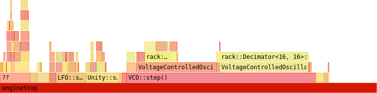
Once profile data is measured, you can view the result in a flame graph, generated by your favorite profiler visualization software. The width of each block, representing a function in the call tree, is proportional to the function’s runtime, so you can easily spot bottlenecks.
Mathematical optimization
If a bottleneck of your code is the evaluation of some mathematical concept, it may be possible to obtain huge speedups of 10,000 or more by simply using another mathematical method. If overhauling the method is not an option (perhaps you are using the best known algorithm), speedups are still possible through a bag of tricks.
- Store frequently re-evaluated values in variables so they are evaluated just once.
- Move expensive functions to lookup tables.
- Approximate functions with polynomials or rational functions, using Horner’s method, Estrin’s scheme, and/or Padé approximants.
- Reorder nested
forloops to “transpose” the algorithm.
Remember that it is important to profile your code before and after any change in hopes of improving performance, otherwise it is easy to fool yourself that a particular method is faster.
Compiler optimization
Compiler Explorer (Note that Rack plugins use compile flags -O3 -march=nehalem -funsafe-math-optimizations.)
TODO
Memory access
TODO
Vector instructions
In 2000, AMD released the AMD64 processor instruction set providing 64-bit wide registers and a few extensions to the existing x86 instruction set. Intel then adopted this instruction set in a line of Xeon multicore processors codenamed Nocona in 2004 and called it Intel 64. Most people now call this architecture x86_64 or the somewhat non-descriptive “64-bit”.
The most important additions to this architecture are the single instruction, multiple data (SIMD) extensions, which allow multiple values to be placed in a vector of registers and processed (summed, multiplied, etc) in a similar number of cycles as processing a single value. These extensions are necessary for battling the slowing down of increases in cycle speed (currently around 3GHz for desktop CPUs) due to reaching the size limits of transistors, so failure to exploit these features may cause your code to run with pre-2004 speed. A few important ones including their first CPU introduction date are as follows.
- MMX (1996) For processing up to 64 bits of packed integers.
- SSE (1999) For processing up to 128 bits of packed floats and integers.
- SSE2 (2001) Extends SSE functionality and fully replaces MMX.
- SSE3 (2004) Slightly extends SSE2 functionality.
- SSE4 (2006) Extends SSE3 functionality.
- AVX (2008) For processing up to 256 bits of floats.
- FMA (2011) For computing
for up to 256 bits of floats. - AVX-512 (2015) For processing up to 512 bits of floats.
You can see which instructions these extensions provide with the Intel Intrinsics Guide or the complete Intel Software Developer’s Manuals and AMD Programming Reference.
Luckily, with flags like -march=nehalem or -march=native on GCC/Clang, the compiler is able to emit optimized instructions to exploit a set of allowed extensions if the code is written in a way that allows vectorization.
If the optimized code is unsatisfactory and you wish to write these instructions yourself, see x86 Built-in Functions in the GCC manual.
Remember that some of your targeted CPUs might not support modern extensions such as SSE4 or AVX, so you can check for support during runtime with GCC’s __builtin_cpu_supports and branch into a fallback implementation if necessary.
It is often preferred to use the more universal _mm_add_ps-like function names for instructions rather than GCC’s __builtin_ia32_addps-like names, so GCC offers a header file x86intrin.h to provide these aliases.